Few days back, I was talking to my team on GPU optimization and then worked on a quick fundamentals blog, then thought of sharing it via a blog, so here it goes.
1. Why GPUs?
A CPU and GPU are designed for somewhat different workloads.
A CPU is optimized for getting a relatively small number of complicated tasks completed quickly.
A GPU is optimized for executing a very large number of similar operations in parallel.
A simplified way to think about it:
| CPU | GPU |
|---|---|
| Few powerful cores | Many execution units |
| Optimized for latency | Optimized for throughput |
| Large sophisticated caches | Massive parallel execution |
| Great branch prediction | Branch divergence can hurt |
| Complex sequential logic | Large repetitive numerical workloads |
| General-purpose workloads | Matrix/vector/ML workloads |
Consider:
for i in range(1_000_000):
c[i] = a[i] + b[i]
A CPU may divide this work among perhaps a handful of CPU cores.
A GPU can conceptually execute thousands of these additions concurrently.
The key condition is:
There must be enough independent work.
2. CPU vs GPU Execution Model
Suppose we want:
C[i] = A[i] + B[i]
On the CPU we might write:
for i in range(N):
C[i] = A[i] + B[i]
Conceptually:
CPU Core
|
+– A[0] + B[0]
+– A[1] + B[1]
+– A[2] + B[2]
…
On the GPU:
Thread 0 → A[0] + B[0]
Thread 1 → A[1] + B[1]
Thread 2 → A[2] + B[2]
Thread 3 → A[3] + B[3]
…
Thread 999999 → A[999999] + B[999999]
The GPU programming model is therefore built around creating huge numbers of lightweight threads.
3. Basic NVIDIA GPU Architecture
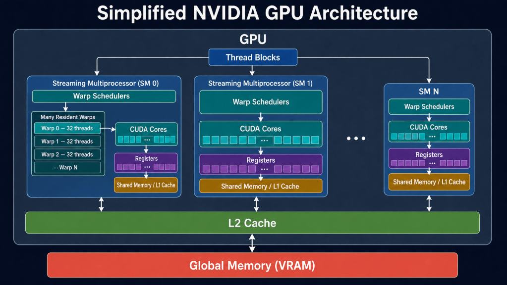
The hierarchy to remember is:
GPU
|
+– Streaming Multiprocessor (SM)
| |
| +– CUDA execution units
| +– Warp schedulers
| +– Registers
| +– Shared Memory / L1
|
+– Streaming Multiprocessor
|
+– Streaming Multiprocessor
|
…
|
+– L2 Cache
|
+– Global GPU Memory
Streaming Multiprocessor — SM
An SM is one of the main computational building blocks of the GPU.
Each SM contains resources used to execute many GPU threads:
- execution units
- warp schedulers
- registers
- shared memory
- cache
You normally don’t assign work directly to individual CUDA execution units.
Instead you launch thousands of threads and the GPU schedules them onto SMs.
4. Thread → Block → Grid
CUDA organizes work as:
Grid
|
+– Block 0
| +– Thread 0
| +– Thread 1
| +– …
|
+– Block 1
|
+– Block 2
Example:
kernel<<<1000, 256>>>();
means roughly:
1000 thread blocks
×
256 threads per block
=
256,000 threads
The GPU schedules blocks across available SMs.
5. Warp
This is one of the most important GPU concepts.
Threads are scheduled in groups called warps.
On NVIDIA GPUs:
1 warp = 32 threads
Conceptually:
Warp
|
+ Thread 0
+ Thread 1
+ Thread 2
…
+ Thread 31
These threads execute instructions together.
This architecture is often described as SIMT — Single Instruction, Multiple Threads.
6. Warp Divergence
Warp divergence can occur when threads within the same warp execute different amounts of workloads, example: a loop for different numbers of iterations.
Suppose each GPU thread processes one customer’s purchase history:
int customer = blockIdx.x * blockDim.x + threadIdx.x;
int purchaseCount = numberOfPurchases[customer];
float total = 0;
for (int i = 0; i < purchaseCount; i++) {
total += purchases[customer][i];
}
Customers may have purchase histories of different lengths:
| Thread | Number of purchases | Loop iterations |
| Thread 0 | 2 | 2 |
| Thread 1 | 5 | 5 |
| Thread 2 | 20 | 20 |
| Thread 3 | 100 | 100 |
| … | … | … |
| Thread 31 | 4 | 4 |
All 32 threads in the warp begin execution together, but they finish at different times:
Iterations 1–2: Most or all threads are active
Iterations 3–5: Thread 0 is inactive
Iterations 6–20: More threads become inactive
Iterations 21–100: Most threads are inactive
Final iteration: Only Thread 3 may still be active

The warp must continue executing until the thread with the longest purchase history finishes. Threads that complete earlier remain inactive during the remaining iterations.
This wastes GPU execution capacity. For example, if only one thread is still active, one execution lane performs useful work while the other 31 lanes remain idle.
This is warp divergence.
Therefore:
GPUs work best when neighboring threads perform similar work.
Potential Optimization
Group customers with similar purchase-history lengths before processing them:
Warp 0 → Customers with 0–8 purchases
Warp 1 → Customers with 9–32 purchases
Warp 2 → Customers with 33–128 purchases
Threads within each warp will then perform a more similar amount of work, keeping more execution lanes active.
Key Takeaway
Warp divergence occurs whenever threads within the same warp follow different execution timelines—not only when the code contains an if/else statement.
GPUs perform best when threads in the same warp execute similar instructions for approximately the same amount of time.
7. GPU Memory Hierarchy
| Memory | Typical size | Scope | Who manages it? | Relative speed |
| Registers | Tens to hundreds of KB per SM | Private to each thread | Compiler and hardware; indirectly influenced by variables in the kernel | Fastest |
| Shared Memory | Tens to hundreds of KB per SM | Shared by threads in the same thread block | Programmer explicitly allocates and accesses it | Very fast |
| L1 Cache | Tens to hundreds of KB per SM; often shares capacity with shared memory | Used by threads running on the same SM | Hardware automatically caches data | Very fast |
| L2 Cache | Several MB to tens of MB across the GPU | Shared by all SMs | Hardware automatically caches data | Fast |
| Global GPU Memory (VRAM) | Several GB to over 100 GB | Accessible by all threads and the CPU through transfers or unified-memory mechanisms | Programmer/runtime allocates it; hardware serves accesses | Slowest GPU memory, but largest |
Registers
Fastest storage.
Generally private to a thread.
Example:
float sum = 0;
sum may live in a register.
Shared memory
Shared between threads within a thread block.
Extremely useful when several threads repeatedly access the same piece of data.
But shared memory is limited.
You cannot normally put a giant vector into shared memory.
L1 / L2 cache
Hardware-managed caches.
Frequently reused values may automatically benefit from them.
Global memory
The GPU’s large device memory.
Much larger, but expensive relative to registers/shared memory.
Many GPU optimization problems are really:
How do we minimize expensive memory traffic?
8. Memory Coalescing
Imagine 32 threads in a warp.
Good access:
Thread 0 → A[0]
Thread 1 → A[1]
Thread 2 → A[2]
…
Thread 31 → A[31]
The addresses are contiguous.
The GPU can service these efficiently using a small number of memory transactions.
Bad access:
Thread 0 → A[10]
Thread 1 → A[9004]
Thread 2 → A[47]
Thread 3 → A[500000]
…
Now memory accesses are scattered.
This generally creates more memory transactions and lower effective bandwidth.
This concept is called memory coalescing.
9. Compute-Bound vs Memory-Bound
A GPU performs two broad kinds of work:
- Moving data from GPU memory to its processing units.
- Performing computations such as multiplication and addition.
Performance depends on which one becomes the bottleneck.
Compute-Bound: Matrix Multiplication
Consider dense matrix multiplication:
C=A×B
A value loaded from A can be reused to calculate multiple elements of C. The same is true for values from B. GPUs load small blocks of both matrices into fast on-chip memory and reuse them for many multiply-add operations.
This creates high arithmetic intensity:
Arithmetic Intensity =
Number of arithmetic operations / Bytes transferred from memory
In other words, the GPU performs a large amount of computation for each byte it reads. The main limit may therefore become how quickly its CUDA cores or Tensor Cores can perform calculations. This is called a compute-bound workload.
Memory-Bound: Sparse Matrix-Vector Multiplication
Now consider:
y=A x
where A is sparse. For every non-zero value, the GPU typically must:
- Read the matrix value.
- Read its column index.
- Use the index to locate and read a value from x.
- Perform one multiplication and one addition.
This requires several memory reads for only a small amount of arithmetic. The irregular column indices may also cause threads to access unrelated memory locations, reducing cache effectiveness and memory-access efficiency.
The GPU’s computational units can therefore spend much of their time waiting for data. Adding more cores or increasing compute capacity will not help much because computation is not the bottleneck. Performance is limited by how quickly memory can supply data, making SpMV (Sparse Matrix multiplied by Vector) frequently memory-bandwidth-bound.
10. Sparse Matrix Example
Consider:
A =
[ 10 0 0 2 ]
[ 0 3 0 0 ]
[ 4 0 5 0 ]
[ 0 0 0 7 ]
Most values are zero.
Storing all 16 values is wasteful.
Instead we can use CSR.
CSR — Compressed Sparse Row
We store three arrays.
data
[10, 2, 3, 4, 5, 7]
indices
Column of each value:
[0, 3, 1, 0, 2, 3]
indptr
Where each row begins:
[0, 2, 3, 5, 6]
Therefore row 0 is:
data[0:2]
=
[10,2]
indices[0:2]
=
[0,3]
11. Sparse Matrix × Vector
Suppose:
x =
[1]
[2]
[3]
[4]
We want:
y = A × x
Row 0:
10 × x[0] + 2 × x[3]
= 10 × 1 + 2 × 4
= 18
Every row can be calculated independently.
That makes SpMV naturally parallel.
12. Simple GPU Implementation
A very simple kernel could assign:
one row → one GPU thread
For example:
row = thread_id
sum = 0
for j = indptr[row] to indptr[row+1]:
col = indices[j]
sum += data[j] * x[col]
y[row] = sum
With 1 million rows:
1,000,000 GPU threads
This sounds ideal.
But several problems appear.
13. Problem #1 — x Has Irregular Memory Access
Look at:
x[indices[j]]
indices[j] might be:
5
987
3
400000
17
…
So neighboring threads could fetch completely unrelated locations of x.
This hurts memory coalescing.
Some values may still hit the hardware caches, but access locality depends heavily on the sparse matrix structure.
14. Why Not Copy x Into Shared Memory?
A common first thought is:
Put x into shared memory because shared memory is fast.
This only works when the working portion of x is small enough.
For a large vector:
x = millions of floats
shared memory per block is far too small to hold the whole vector.
Instead we generally rely on:
- L1/L2 cache
- locality
- tiling where applicable
- better matrix organization
- specialized kernels
The important distinction is:
cache → hardware managed
shared memory → programmer managed
15. Problem #2 — Uneven Rows
Imagine:
Row 0 → 2 non-zero values
Row 1 → 5
Row 2 → 400
Row 3 → 3
If every thread gets one row:
Thread 0 finishes quickly
Thread 1 finishes quickly
Thread 2 keeps working
Thread 3 finishes quickly
Threads sharing a warp may finish at very different times.
That causes poor utilization.
16. Better Approach — Warp Per Row
Instead of:
1 thread → 1 row
we can sometimes use:
1 warp → 1 row
Example:
Row has 128 nonzeros
32 warp threads
Thread 0 → elements 0,32,64,96
Thread 1 → elements 1,33,65,97
…
Thread 31 → elements 31,63,95,127
Each thread calculates a partial result.
Then we perform a warp reduction:
partial sums
↓
warp reduction
↓
final row value
Now the work for a long row is distributed among many threads.
ELLPACK (ELL): Regularizing Sparse Rows
Another optimization is the ELL sparse-matrix format. ELL stores every matrix row using the same fixed number of slots.
Suppose the longest row has four non-zero values:
Original rows:
Row 0 → 3 values
Row 1 → 1 value
Row 2 → 4 values
ELL pads shorter rows with zeros:
| Row | Values | Column indices |
| 0 | 5, 8, 2, 0 | 0, 3, 6, 0 |
| 1 | 7, 0, 0, 0 | 2, 0, 0, 0 |
| 2 | 4, 1, 9, 6 | 0, 2, 5, 7 |
Sliced ELL: Group Rows of Similar Length: Standard ELL pads every row to the length of the longest row in the entire matrix. A single unusually long row can therefore cause excessive padding.
Instead, divide the matrix into groups—or slices—of rows with similar numbers of non-zeros. Each slice uses its own ELL width.
For example:
| Slice | Row lengths | ELL width after padding |
| Short rows | 3, 4, 4, 5 | 5 |
| Medium rows | 14, 15, 16, 16 | 16 |
| Long rows | 61, 64, 67, 70 | 70 |
Without grouping, standard ELL would pad every row to 70 elements. With sliced ELL, each row is padded only to the maximum length within its slice.
The slices can then use different execution strategies:
- Short rows: one thread processes one row.
- Medium rows: several threads cooperate on one row.
- Long rows: one or more warps process one row and combine partial sums using a reduction.
Rows are usually reordered or grouped by similar length before creating the slices. The final output must use a permutation map to restore the original row order.
Warp vs. SM Assignment
Assigning work at the warp level is practical:
Warp 0 → one long row
Warp 1 → another long row
Warp 2 → several short rows
However, kernels do not normally assign rows directly to a physical Streaming Multiprocessor (SM). Instead, they create thread blocks, and the GPU scheduler places those blocks on available SMs.
This approach provides:
- Less zero padding than standard ELL.
- Less warp divergence because grouped rows have similar workloads.
- Better load balance between warps.
- More coalesced access for matrix values and column indices.
The trade-offs are preprocessing, row-reordering metadata, and possible imbalance when a slice still contains an unusually long row.
17. GPU Optimization Checklist
When examining a GPU kernel, ask these questions in roughly this order.
1. Is there enough parallelism?
Bad:
100 operations
Good:
10,000,000 independent operations
2. Are memory accesses coalesced?
Try to make neighboring threads access neighboring memory.
3. Is the kernel compute-bound or memory-bound?
If memory-bound:
making multiplication faster
may do almost nothing.
You need to reduce or improve memory traffic.
4. Is there warp divergence?
Look for:
if
switch
loops with different lengths
across threads in the same warp.
5. Is there load imbalance?
SpMV example:
row 1 → 4 values
row 2 → 500 values
6. Can data be reused?
Possible locations:
Registers
Shared Memory
Cache
7. Are CPU ↔ GPU copies dominating?
This is often overlooked.
Bad:
CPU → GPU
kernel
GPU → CPU
CPU → GPU
kernel
GPU → CPU
Better:
CPU → GPU
kernel
kernel
kernel
kernel
GPU → CPU
Keep data on the GPU whenever practical.
8. Is the workload large enough?
GPU kernel launches and transfers have overhead.
For tiny workloads:
CPU may win.
9. Are we using existing optimized libraries?
Before writing a custom sparse kernel, consider:
cuSPARSE
For dense linear algebra:
cuBLAS
For deep learning:
cuDNN
Highly tuned libraries will often beat straightforward custom implementations.
18. Ads Example — CTR Prediction
Imagine every ad impression contains:
member_id
ad_id
campaign_id
device
country
historical CTR
context features
A model could look like:
member_id ─────→ embedding ──┐
|
ad_id ─────────→ embedding ──|
|
campaign_id ───→ embedding ──|→ concatenate → MLP → P(click)
|
dense features ──────────────┘
Training this model involves two interesting GPU workloads.
Embedding lookups
embedding[user_id]
embedding[ad_id]
These accesses can be irregular and memory-heavy.
This has an interesting similarity to SpMV:
SpMV:
x[indices[j]]
Ads model:
embedding[id]
Both demonstrate that memory behavior matters.
Dense layers
The MLP performs operations approximately like:
batch × weights
These are dense matrix multiplications and are an excellent fit for GPU parallelism.
21. GPU Training Optimization
For an ads model we can improve performance using:
Larger batches
256
1024
4096
8192
Larger batches generally expose more parallel work until another resource becomes limiting.
Mixed precision
Instead of exclusively FP32:
FP16 / BF16
can reduce memory traffic and enable specialized GPU acceleration where supported.
Keep model on GPU
Avoid repeatedly moving model parameters between CPU and GPU.
Efficient input pipeline
Use:
multiple data-loader workers
pinned memory
prefetch
asynchronous transfers
so that the GPU does not spend time waiting for the CPU.
Kernel fusion
Instead of:
kernel A
write memory
kernel B
read memory
kernel C
write memory
fusing operations may reduce launch overhead and intermediate memory traffic.
22. The Mental Model to Remember
The most important GPU optimization equation is not:
MORE CUDA CORES = FAST
It is:
Performance
=
parallelism
×
efficient memory access
×
good utilization
×
enough work
When debugging GPU performance, think:
GPU slow
|
+————+————+
| | |
Compute Memory Utilization
| | |
too much math bandwidth divergence
wrong precision latency imbalance
small workload
For SpMV specifically:
Parallelism ✓
Lots of threads
Arithmetic low
Memory traffic high
x access irregular
Row lengths potentially irregular
Result:
usually a memory-bound GPU problem
That makes SpMV an excellent example for learning GPU optimization.
23. Examples
Basis addition link
Sparse Matrix × Vector (SpMV) link
Ads CTR link
Nvidia CUDA intro link

